Electrical Reliability – An Introduction
Electrical Reliability is something that tends to be talked about often in electrical design, but usually only in general terms like an N-1 outage or an N-2 outage. This approach is OK in terms of simple reliability, for redundancy purposes, but it doesn’t really consider the issue of how reliable a system actually is and how this reliability (or lack of) can translate into lost revenue. Intrigued? Then read on.
As a former Oil & Gas engineer, I find it strange that reliability and availability is almost never talked about in renewable and industrial design. Perhaps it is because the UK Grid is very reliable and when faults do occur there are a lot of companies out there that can respond and help fix problems quickly and efficiently. But by not considering electrical reliability and availability of a system design, many developers are missing a trick as spending some time assessing the system design can have a major impact on a systems performance, the revenue generated and in many cases a companies reputation.
In this article we will just take a simple look at electrical reliability and availability, and skip the more complex maths, but it is worth noting that there is a formal analysis method defined in IEEE 493 – IEEE Recommended Practice for the Design of Reliable Industrial and Commercial Power Systems. I will write a separate article about this process, as it is an interesting, but complex area and apply it to Battery Storage where there are specific reliability and availability targets to meet.
For this article we are going to focus on Solar PV systems as these are common and often designed the same way, but the general thought process can be applied to any industrial system; for a similar reason we are also going to focus just on the HV, and assume the transformer and inverter design is the same at all plants – but of course we could expand our analysis to consider the reliability/ availability and cost benefits of string inverters vs central inverters. The other thing to note in Solar PV is that if a failure occurs, then the failure of one component does not (usually) cause loss of the whole system, but instead reduces its overall output.
Part 1 – Reliability based on an ‘N’ concept
First let’s talk about electrical reliability in general terms of N, N-1 and N-2. These are basic concepts that are based on the idea that for an ‘N’ design, an outage (planned or unplanned) will cause the system to lose power – these kind of schemes are typical for low cost low reliability schemes, where an outage doesn’t cost much money or cause any major inconvenience. In an N-1 design you can have an outage (planned or unplanned) on the system, and you can still deliver power to where it is needed, this system configuration comes in many different guises, such as ring system, dual redundant transformers and so on, but they all have the basic same idea – if something is unavailable you can still continue to operate.
An N-2 design is a scheme where you can have two outages (planned or unplanned), and still deliver power, these schemes are commonly used in UPS configurations, or on an islanded power system, or microgrid, where a unit could be out of service for a while for a planned outage, and the system still needs to be able to withstand an unplanned outage. For the rest of this paper we can forget about N-2 designs, as they are a bit unusual; and require some special considerations.
So first let’s take a look at a typical simplified Solar PV scheme shown below in Figure 1. We can see here that if the main MV Cable 1 faults, or RMU #1 has a catastrophic failure the whole site will be lost, if MV-Cable #2 faults or Station #2 faults then 75% of the site is lost and so on. In all cases, if a transformer fails, only a local inverter group is lost. This is a classic ‘N’ design configuration. For our test case lets assume that each Inverter Station is identical to the others and rated at 2.5MW each, giving a total rating of 10MW.
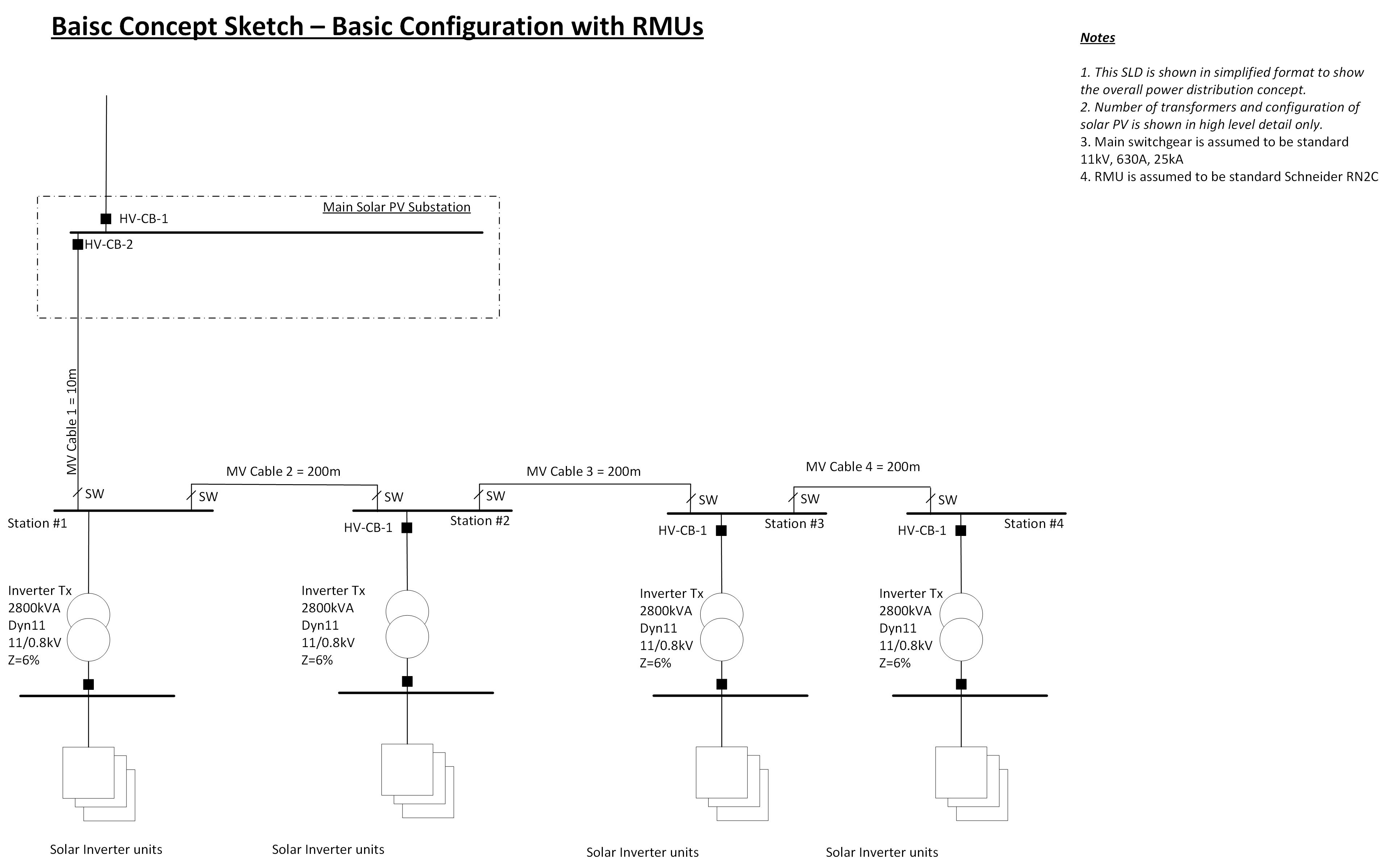
Figure 1 – Radial Feed
If we want to improve our electrical reliability, we have a simple option. We install an extra circuit breaker on the main switchboard, another 800m of cable and a switch on the end RMU. The revised system can now be seen in Figure 2, and it can be observed that the system now has an N-1 level of redundancy; this means that a cable fault on any part of the network won’t affect overall production, and a catastrophic RMU failure will only take a single inverter station out of service.
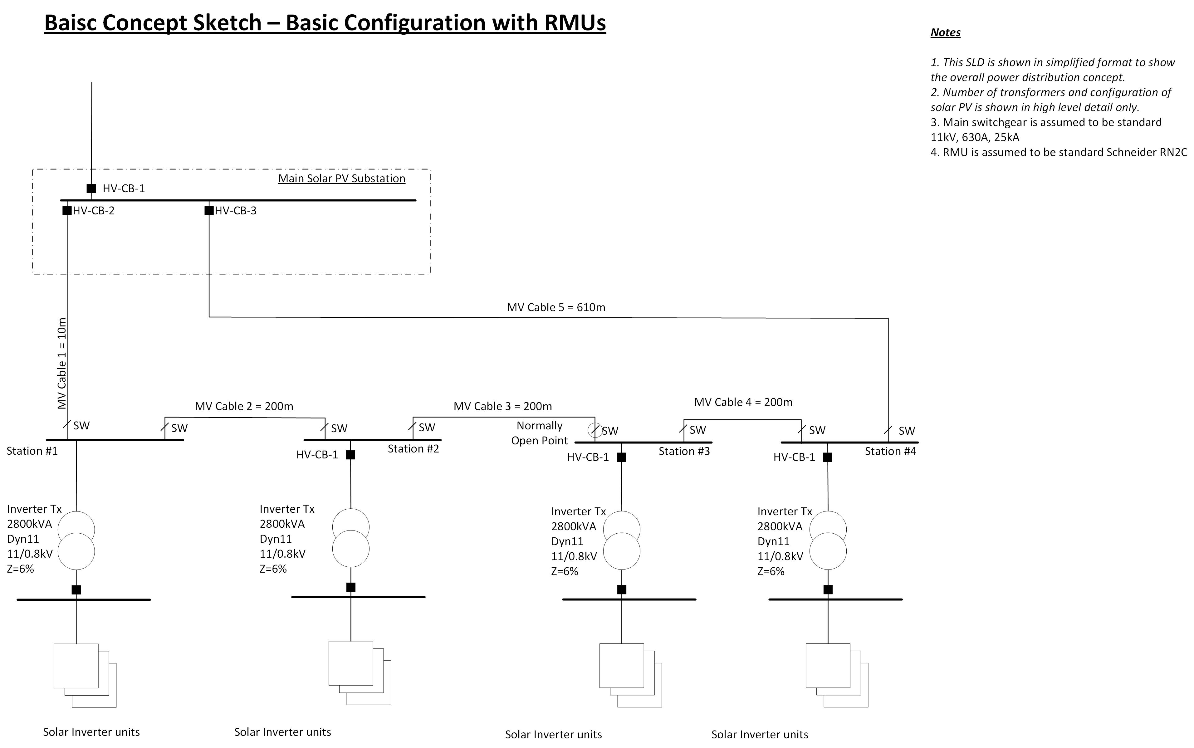
Figure 2 – Simple Ring
This seems like a simple trade off the cost of the extra equipment, vs the cost of forced downtime due to a fault. We will come back to this in a bit, but first let’s look at different configuration that for some reason is almost never used in Solar PV. It is based on an N design, so in principle has the same level of redundancy as Figure 1, but in practice it gives a much better performance than our original design. This can be seen below in Figure 3, where each inverter station is given its own dedicated feeder from the main switchboard. Figure 3 is technically a radial system, but we can refer to it as a individual feeder design, or a ‘star’ network.
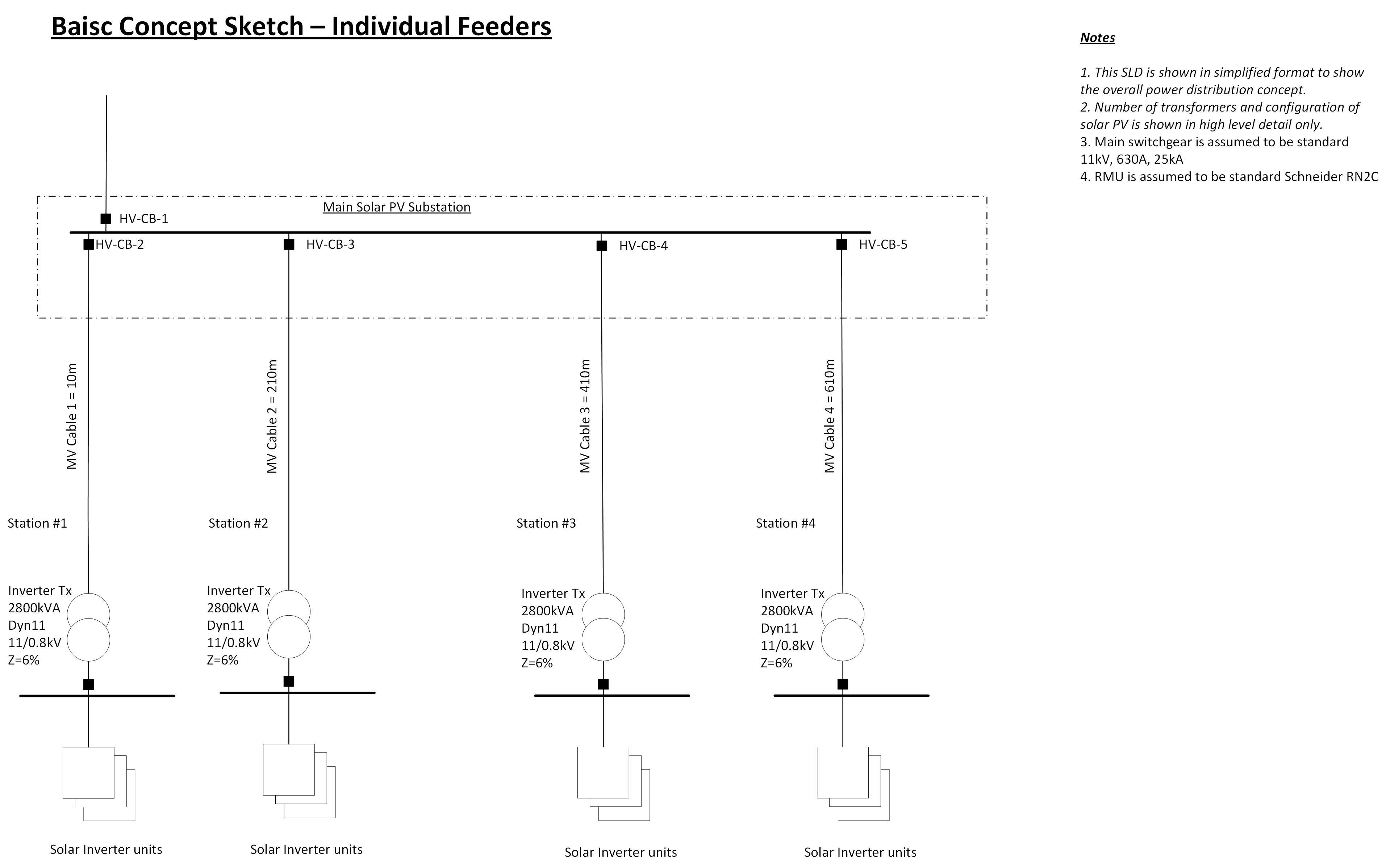
Figure 3 – Independent Radial Feeders
Inherently it can be seen that this system should be more reliable and robust than Figure 1, as each inverter is individually supplied; but is it better or worse the Figure 2? On paper, there are more 11kV circuit breakers, and there is more cable, but we have managed to get rid of our RMUs so there may be a cost saving and a reliability improvement as there are less things to go wrong.
Part 2 – CAPEX Costs
Next it is useful if we compare our 3 options above, in terms of CAPEX (Capital Expenditure) costs. I don’t have lots of accurate cost figures to hand, so I have put in some typical ones, and the reader should take them with a pinch of salt. We can compare the three options, using a simple Excel spreadsheet to end up with something that might look like below.

Figure 4 – Cost Comparison
Surprisingly, Option 1 and Option 3 come out at a very similar basis, because Option 3 saves the RMU cost but increases the cable cost. Option 2 doesn’t look too competitive as its similar to Option 1, but with an extra 11kV breaker and a run of cable.
What is interesting in the above is that the most reliable design in our test case came out the cheapest and was pretty similar to the conventional design. Of course, in the above configuration, cable costs are the key variable and sites with small runs and simple geography favor the parallel feeder design, whilst if the cable lengths increase significantly then the economics will change.
Part 3 – Lost Revenue
This is the bit where non-engineers tend to get interested – and rightly so, if you are investing £XXXm in a new generation scheme, then you want to maximize your Return on Investment (RoI), achieve the most cost effective design and prevent outages from causing lost revenue.
Sticking with our Solar PV design, the actual revenue cost of generation varies significantly depending on the type of contract and how far ahead the energy is traded. However, in very simple terms, the approximate cost per MWh of generation can be assumed as around £45 per MWh[1], which is equivalent to 4.5p per kWh.
For simplification purposes, assume that all inverter stations are rated at 2500kW and we are ignoring reactive power generation and costs we get from being available, or any other subsidies. Thus, for an energy cost of 5p kWh, the lost revenue per hour is simply £112.5 / inverter station (2500kW *4.5p / kWh). However, as solar PV arrays only produce power during sunlight hours, and less energy during early morning and late evening, this figure can be adjusted down by a factor of say 10 hrs in 24 i.e. 40%. So, if we know that the MTTR per inverter station is an average of 56 hours, we can write: Loss per Station = £6,300 / event and Loss Daylight Hours Weighted per Station (LWS)= £2,520 / event.
Armed with the above information we can do some very simple number crunching for the three cases we discussed earlier. We need to do a bit of maths to give some weightings to thing and make a few assumptions, but they should help us get a clearer picture of what is going on. Recapping from earlier, it can be seen that a major failure of an RMU or cable associated with the PV1 unit will lead to loss of all inverter stations. A major failure occurs on PV2 unit switchgear, then PV2, PV3 and PV4 would all be unavailable until the system is repaired, and there would be a reduction in the available power output by the plant by 75%. Similarly, a failure on PV3 switchgear would lead to an available power reduction by 50%.
Probability of Failure and Mean Time to Repair
To put some context into things, we need to have some probabilities for equipment failures and repair rates. This can be a bit of a tricky subject and is a bit too difficult to explain quickly here, but I will put another post together on the subject – for the moment, we can use some reliability and Mean Time To Repair (MTTR) values that I calculated a while ago using the IEEE 493 method. This gives a typical RMU and 200m cable circuit availability of 99.9579% per year, and an associated probability of failure of 0.06289. The probability of failure is the same at each station, the typical MTTR value for this would be 56 hours.
Using some basic maths, we can describe a failure event (E) at each location, in terms of probability and impact i.e. number of inverter stations removed from service for a fault at each location. Therefore, we can consider the lost revenue in the following terms:
Lost Revenue (LR) = Probability (P) * Loss Weighted Per Station(LWS) * Number of Stations Affected (N).
If we tidy things up a bit and use a simple Excel model, we end up with something like Figures 5, 6 & 6 shown below (one for each of our earlier cases). In Figure 5 we can see that the consequential loss starts to build up, as a failure in the wrong place can take out the whole system.
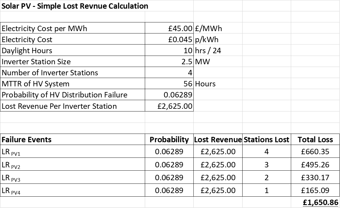
Figure 5 – Lost Revenue for a Radial System
Figure 6 (below), is very similar to Figure 5, but our ring system means that a fault on any part of the network apart from the main switchboard, will only result in loss of a single inverter station. So the potential lost revenue per year is reduced by around 40%.

Figure 6 – Lost Revenue for a Ring System
In the last scenario, we have reduced the probability of failure my a significant margin, as there are no longer any RMUs, but we have increased the MTTR of the system, as an HV failure is now likely to take longer to repair. We now end up with an even lower potential lost revenue figure.
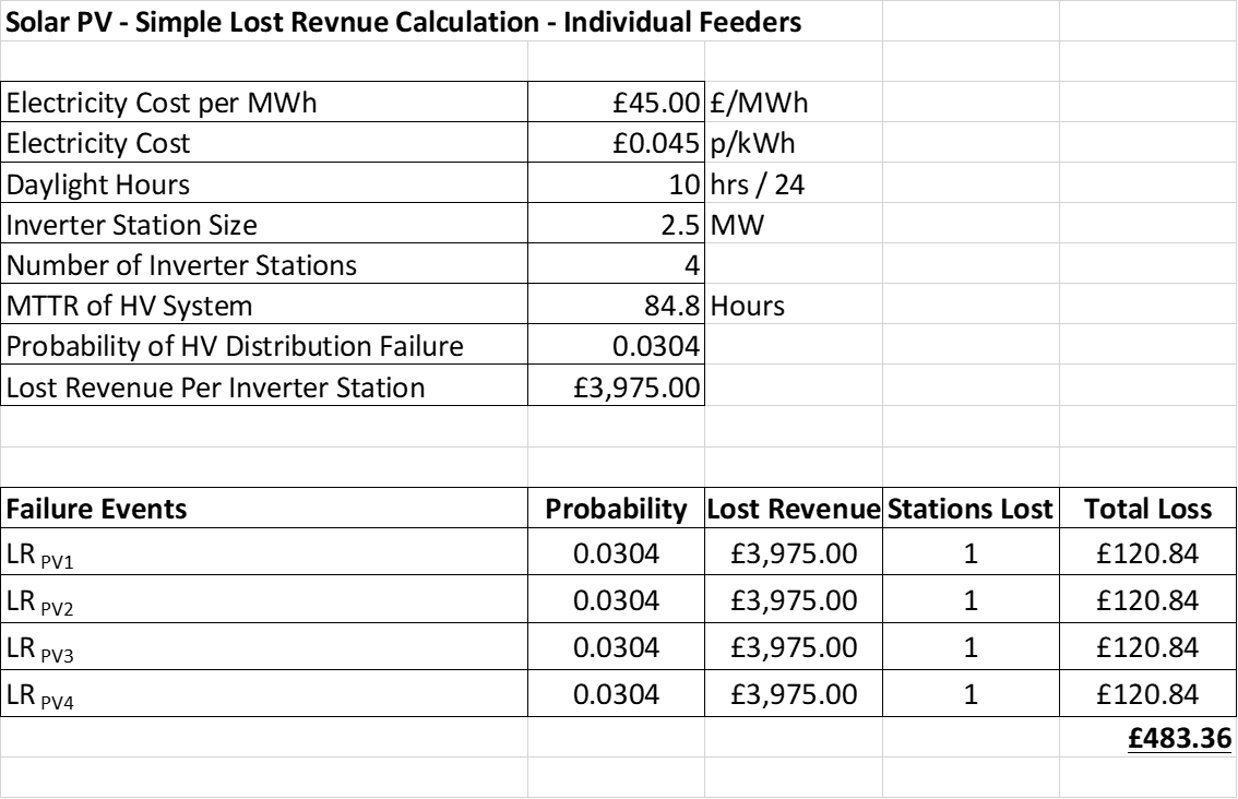
Figure 7 – Lost Revenue for an Independent Feeder System
It is noted of course that the above figures are average lost revenue per year. For designs that use larger inverters, or more inverters on a single radial feeder, then the potential losses will be higher, whilst designs that have smaller inverters or a more distributed design will have lower losses.
Summary
Depending on the HV power system distribution design, failures at certain points can have a huge impact i.e. a fault in the wrong place can taking out a whole site and mean a substantial loss of production and revenue until it is repaired and therefore electrical reliability is a key issue to understand. Conventional simple radial design with RMUs are cheap and easy, but there are other alternative designs that can be only slightly more expensive and give a significant improvement in reliability.
In general, what we find is that a carefully laid out ring system, which optimizes cable lengths, or a ‘star’ type configuration with individual feeders can offer increased availability and resilience to faults for little extra cost. The question that needs analysis on a case-by-case basis, is if the extra equipment cost is justified by the increase in reliability and lost revenue.
The financial numbers we have used here are pretty simple, and don’t take into account the fact that electricity price is volatile, summer and winter loads and so on. Longer term financial considerations like discounted cash flows, on the probable increasing cost of electricity prices are also not considered and these factors could make some interesting changes to system design.
As with all engineering design issues though, we have to ask ourselves if the additional electrical reliability and potential revenue saving justifies the additional equipment cost. In practice this is very site specific and depends on the revenue modelling used as the relative cost of the equipment. Potential investors are also likely to be interested in such analysis and these kind of design analysis, can help future asset sale of a plant.
[1] Based on typical Energy UK wholesale market figures