Ross Falconer, Head of Power Systems, Aurora Power Consulting
Currently we are working on an innovation project with Northern Power Grid (NPG) to develop their policy for assessing voltage fluctuations on the grid caused by Battery Energy Storage Systems (BESS’s).
As we decarbonise the grid and move away from traditional generation sources like coal and gas, other forms of energy storage are needed to control the system frequency by importing and exporting power in response to frequency changes on the grid. BESS’s are good at this and are currently quite economical, which is why we are seeing a lot of grid-scale BESS’s applying to get connected. However, BESS’s can have an adverse effect on grid voltages, as they ramp from importing power to exporting power, they can cause voltage to fluctuate.
As part of our innovation project with NPG, we have been very interested in trying to quantify just how much the grid frequency changes over time. Once we know how much variation there is in grid frequency, we will then be able to predict how BESS’s will respond to those changes by ramping their power, and hence we can then determine by how much the voltage will fluctuate due to BESS activity.
We expect that most of the time the grid frequency will be approximately 50 Hz with some small variation around that. At a first guess, you’d expect the grid frequency to follow a normal distribution curve centred on 50 Hz. We were very surprised then we started to look at the distribution of grid frequency recorded by the Electricity System Operator (ESO) from last year (2023), as shown in the plot below:
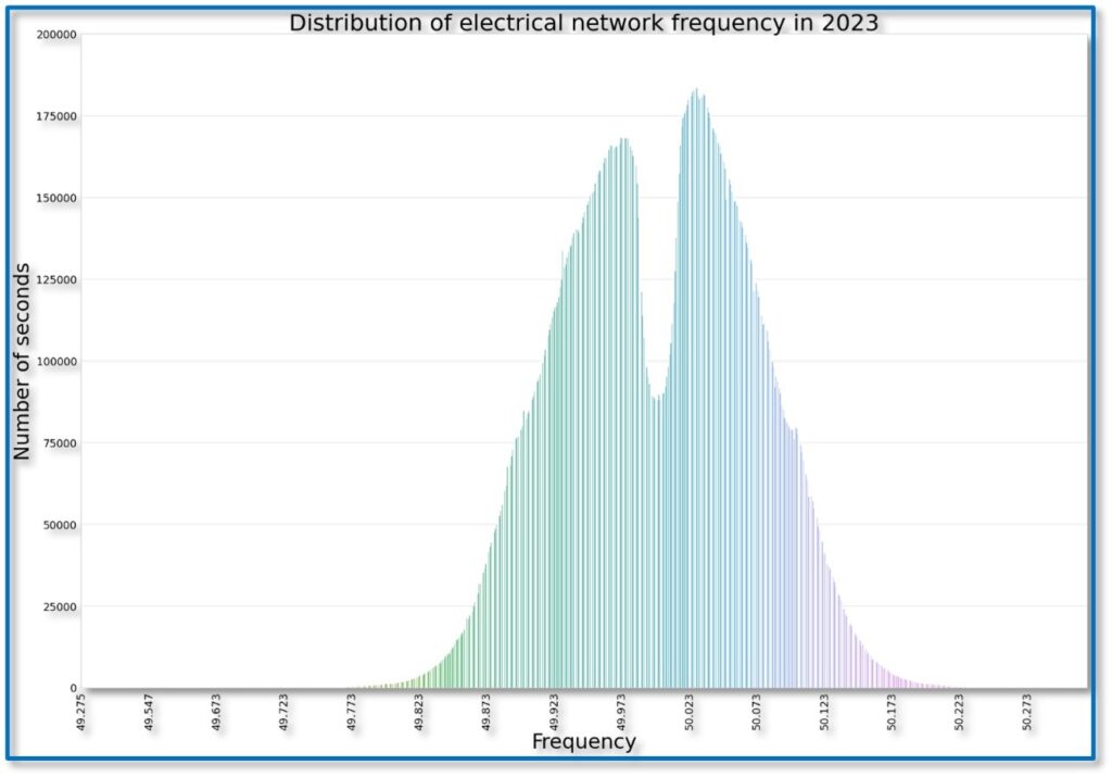
It does not follow a normal distribution! Yes, it is centred around 50 Hz, but there is a strange drop in the middle of the distribution. Between about 49.85 Hz and 50.15 Hz, the typical bell-curve shape had a chuck missing from it, which means that actually most of the time the system frequency is running slightly below or slightly above 50 Hz.
Here at Aurora, we have been scratching our heads trying to explain why the frequency distribution does not follow a normal distribution. Possible theories that we had were:
- Perhaps this is just an artefact of the sampling method that ESO are using. Maybe their recording devices don’t trigger unless there is a move away from 50 Hz?
- My theory was that maybe ESO deliberately run the system frequency high for a while when they know a large load is going to come on. For example, they run it high before the evening load comes on, and then deliberately run the frequency low during the middle of the night to ensure the cumulative change in frequency over the day is zero.
- Our python statistical analysis whiz, Hesam, thought it might be to do with the deadband in frequency response services. I wasn’t so sure, but it was worth exploring.
So, what is this mysterious deadband in frequency response services? For a start, what are frequency response services?
Frequency response services are a commercial market that the ESO uses to control system frequency. When the frequency goes high this is a sign that there is too much generation on the grid, ESO wants providers to import power to bring the frequency back down towards 50 Hz. Conversely, when the frequency goes low this is a sign that there is too much load on the grid and ESO needs providers to start generating power to bring the frequency back up.
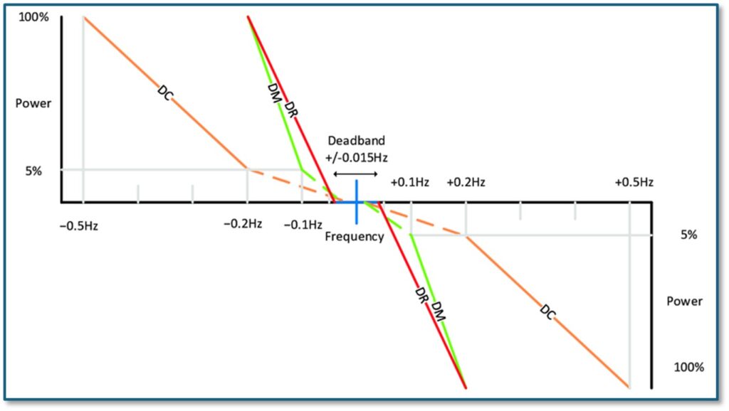
There are two main services that do the bulk of the work: Dynamic Regulation and Dynamic Moderation. DR and DM for short. There is also Dynamic Containment (DC), but that is more of a post-fault response, rather than something which is working all the time. The plot below shows how these services are obligated to import or export power depending on the system frequency.
To understand this plot, I feel the need for an analogy: We can think of the system frequency being like a ball bouncing around, and the DR and DM services being like two springs which try to keep that ball as close as possible to 50 Hz. The ball has some kinetic energy as it jitters about the place. When you turn on the lights on that gives the ball a little kick to the left (lowering the system frequency), when the wind starts blowing hard on a wind turbine that kicks the ball a little to the right (increasing the frequency). Most of the time the ball doesn’t jitter very much, but if something were to go very wrong, for example a large offshore wind farm was to trip out of service, that would give the ball a very big kick to the left. Or if we were exporting a lot of power to another country via one of our undersea cables, and the cable tripped out, that would kick the ball hard to the right.
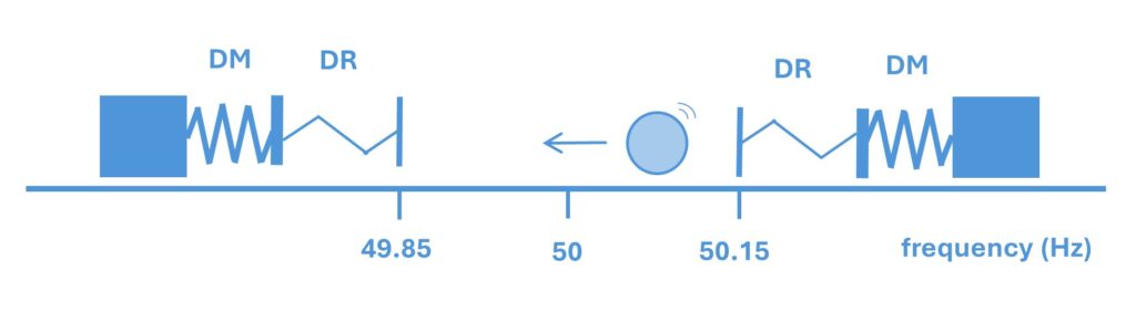
DR is like a little lightweight spring, dealing with the small fluctuations in frequency. DM is like a much harder heavier spring controlling those big fluctuations in frequency.
There is a deadband however, between 49.85 Hz and 50.15 Hz (i.e. +/- 0.015 Hz) DR and DM aren’t required to do anything. So, it’s like the springs controlling the ball don’t extend into the region between 49.85 Hz and 50.15 Hz. Could this be enough to explain the missing chunk in the frequency distribution plot above? Possibly, but to me it still didn’t make sense. Why would a deadband cause the system frequency to spend less time at 50 Hz? Looking at the analogy of the ball bouncing around, just because the DR and DM springs don’t extend right into the centre, why should this cause the ball to spend less time in the centre?
After sitting down to a good strong double-shot coconut latte, I had a thought: Maybe the ball isn’t rolling around on a flat surface, maybe the ball is rolling around on a curved surface instead?
What would make the surface curved? To answer this, we can think about the swing equation, which dictates how fast the system frequency changes in response to a mismatch in the power being generated and the power being consumed, that is, dP = Pgenerated-Pconsumed. In this form the swing equation is:

df/dt is our familiar old friend, Rate of Change of Frequency, or RoCoF. And the swing equation says that the rate of change of frequency depends on ΔP multiplied by the frequency. The system inertia is I, which sort of represents the mass of the power system and how sluggishly it will respond to power mismatches.
Now, I’m going to do something a little bit funky and take the derivative of df/dt. That is, I want to find out the rate of change of the rate of change of frequency, or, as I like to call it, the RoCoRoCoF. Taking the derivative of both sides we get:

We can then substitute the expression for RoCoF (df/dt) from equation (1) back into equation (2) to get:

Now, for reasons you’ll see soon, I’m going to put some of that messy stuff which doesn’t depend on time into a constant called k, just to tidy equation (3) up:

Substituting this into (3) yields:

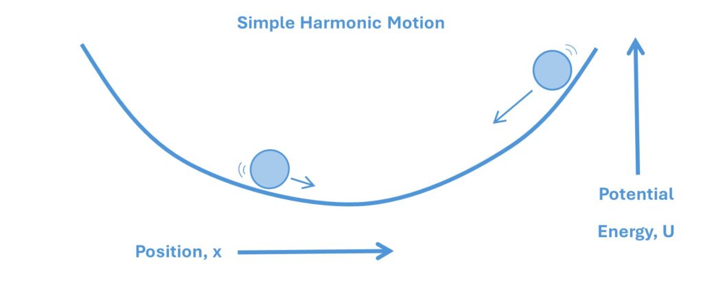
Now does equation (5) remind you of anything, if you think back to A-level physics? The second derivative of frequency, d2f / dt2, is kind of like the acceleration of frequency. If RoCoF is the velocity of frequency, then RoCoRoCoF is like the acceleration of frequency. Hopefully it reminds you of the formula for simple harmonic motion, i.e. the behaviour of a spring:

Where d2x / dt2 is the acceleration, k is the spring constant, m is the mass, and x is the position. Equations (5) and (6) are almost identical if you think of frequency, f, being analogous to position, x. There is one big difference between the behaviour of a spring governed by equation (6) and the behaviour of a power system governed by equation (5) however. There is a negative sign!
The negative sign is what keeps the spring under control. You move the spring away from its initial position and the force acts in the opposite direction to pull the spring back to its equilibrium point. A power system is different however, if you make the frequency go high due to a power imbalance and do nothing to correct that power imbalance, the frequency will keep going even higher in the same direction.
We can think about the potential energy of a spring (or simple harmonic motion in general). The potential energy, U, is given by:

Which is a nice stable parabolic curve. Going back to our ball analogy, if the ball rolls up the hill, its potential energy will increase, and it will roll back down the hill again and come to rest at a stable equilibrium point in the middle.
For the frequency of a power system however, that pesky negative sign means the potential energy, U, is inverted like this:

Now if the ball is at the top of the hill and starts rolling down, it will keep rolling down even further at a faster rate!
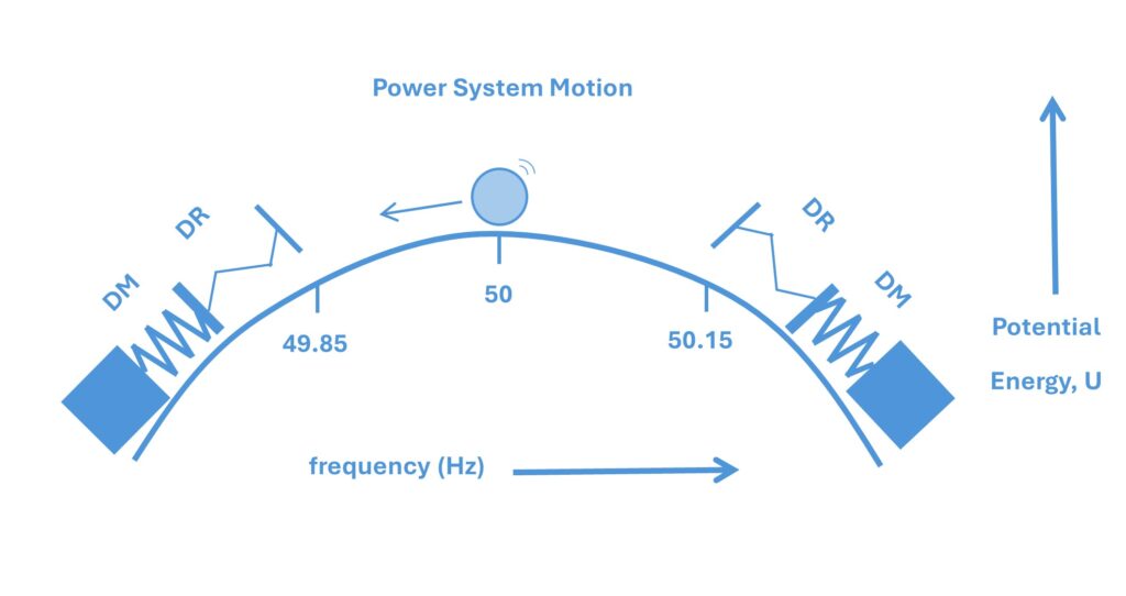
So, we can see that the frequency response services, DR and DM, are controlling the ball to stop it rolling down the hill. This means that 50 Hz is not a stable equilibrium point, it is actually an unstable equilibrium point. This explains the chuck that was missing in the frequency distribution from last year. It doesn’t follow a normal distribution shape because 50 Hz is an unstable equilibrium point.
The ball will spend a lot of its time on one side of the hill e.g. 50.15 Hz, but give it enough of a kick, e.g. everyone go and turn on your kettle during half-time when a big football game is on TV, and the ball will roll over to the other side of the hill and bounce around there for a while. Until it gets a big enough kick to roll back to the other side.
So, the next time someone asks you: What frequency does the GB power system normally run at? Don’t say it is 50 Hz. Say that most of the time it is actually 49.85 Hz or 50.15 Hz.